• 时间序列预测
  • 时间序列的性能评估
  • 时间序列的特征
    • 时间索引特征
    • 滞后特征
  • 趋势
    • 预测未来
    • 高阶 order
  • 季节性
    • 季节规律图
    • 周期图
    • 结合大趋势
  • 依赖过去的特征
    • 自相关函数 ACF
    • 部分相关性函数 PACF
    • 截尾和拖尾
  • 残差
    • 处理油价
    • 处理假日

时间序列可能是目前我遇到的一个比较难的系列，而且我现在只能够说弄懂了一些，还不能够独立完成这样的任务。但是无论如何，我先把这些记录在这里，后面再来补充。

时间序列预测

常规的机器学习一般分为两类，分类和回归，但是时间序列预测看上去却不属于这两类。时间序列一般是时间为索引。

时间序列的性能评估

一般使用 RMSE 来衡量模型的性能，即预测值和目标之间的平方误差根。

时间序列的特征

时间序列一般有两个特征，一个是基于时间索引的特征，一个是滞后特征。

基于时间索引的特征，可以用来估算出时间序列的趋势和季节。

滞后特征是指将过去的目标值当做特征，有时候可能过去的目标值会影响当前的目标值。

时间索引特征

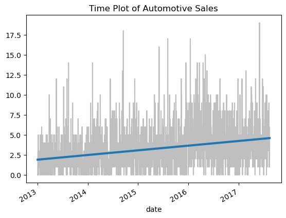
下面一段代码将根据time_step和sales画出他们的线性关系。这里只有time_step这个特征，没有其他的特征进入模型训练。

import pandas as pd
import matplotlib.pyplot as plt
import numpy as np
from sklearn.linear_model import LinearRegression

df = pd.read_csv("train.csv", parse_dates=["date"])
df_automotive = df[(df['store_nbr'] == 1) & (df['family'] == 'AUTOMOTIVE')]
df_automotive = df_automotive.set_index('date').to_period('D')
df_automotive['time_step'] = np.arange(len(df_automotive.index))
y = df_automotive['sales']
X = df_automotive[['time_step']]
model = LinearRegression()
model.fit(X, y)

y_pred = pd.Series(model.predict(X), index=X.index)

plot_params = {'color': '0.75', 'style': '-', 'markeredgecolor': '0.25', 'markerfacecolor': '0.25', 'legend': False}
ax = y.plot(**plot_params)
ax = y_pred.plot(ax=ax, linewidth=3)
ax.set_title('Time Plot of Automotive Sales');

滞后特征

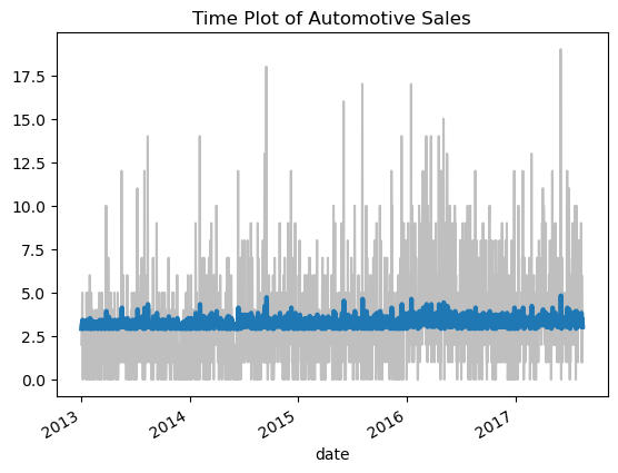
如果将上面的代码改一下，将前一天的sales作为一个滞后特征，然后训练模型。

df_automotive['lag_1'] = df_automotive['sales'].shift(1)
X = df_automotive[['lag_1']].dropna()
y = df_automotive['sales']
y, X = y.align(X, join='inner')

model = LinearRegression()
model.fit(X, y)

y_pred = pd.Series(model.predict(X), index=X.index)

ax = y.plot(**plot_params)
ax = y_pred.plot(ax=ax, linewidth=3)
ax.set_title('Time Plot of Automotive Sales');

趋势

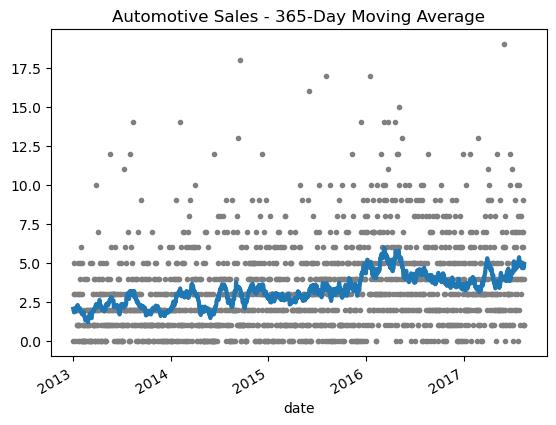
如果我们将Automotive的sales做 30 天的平滑处理，就可以得到下面这样的图，可以从一个比较长的周期看到整个销售的大趋势。

moving_average = df_automotive['sales'].rolling(
    window=30,       # 365-day window
    center=True,      # puts the average at the center of the window
    min_periods=15,  # choose about half the window size
).mean()              # compute the mean (could also do median, std, min, max, ...)

ax = df_automotive['sales'].plot(style=".", color="0.5")
moving_average.plot(
    ax=ax, linewidth=3, title="Automotive Sales - 30-Day Moving Average", legend=False,
);

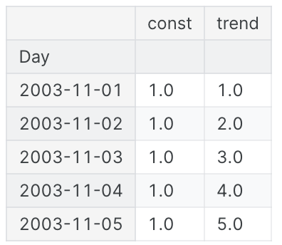
我们可以借助DeterministicProcess算出时间索引特征，而不再需要自己手动计算time_step

from statsmodels.tsa.deterministic import DeterministicProcess

dp = DeterministicProcess(
    index=df_automotive.index,  # dates from the training data
    constant=True,       # dummy feature for the bias (y_intercept)
    order=1,             # the time dummy (trend)
    drop=True,           # drop terms if necessary to avoid collinearity
)
# `in_sample` creates features for the dates given in the `index` argument
X = dp.in_sample()

X.head()

同样也可以画出这个大趋势，和直接用线性模型的效果一样。

from sklearn.linear_model import LinearRegression

y = df_automotive["sales"]  # the target

model = LinearRegression(fit_intercept=False)
model.fit(X, y)

y_pred = pd.Series(model.predict(X), index=X.index)

ax = y.plot(**plot_params)
ax = y_pred.plot(ax=ax, linewidth=3)
ax.set_title('Time Plot of Automotive Sales');

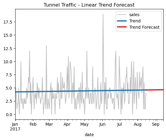
预测未来

DeterministicProcess 能够通过out_of_sample快速算出接下来的 30 天的特征，进而用来预测后面 30 天。

X = dp.out_of_sample(steps=30)

y_fore = pd.Series(model.predict(X), index=X.index)

ax = df_automotive["2017-01-01":]['sales'].plot(title="Automotive Sales - Linear Trend Forecast", **plot_params)
ax = y_pred["2017-01-01":].plot(ax=ax, linewidth=3, label="Trend")
ax = y_fore.plot(ax=ax, linewidth=3, label="Trend Forecast", color="C3")
_ = ax.legend()

高阶 order

如果 order 过高，可能会导致预测值陡然上升或者下降，一般 order 都不要设置太高。

dp = DeterministicProcess(
    index=df_automotive.index,  # dates from the training data
    constant=True,       # dummy feature for the bias (y_intercept)
    order=9,             # the time dummy (trend)
    drop=True,           # drop terms if necessary to avoid collinearity
)
X = dp.in_sample()
y = df_automotive["sales"]  # the target

model = LinearRegression(fit_intercept=False)
model.fit(X, y)

y_pred = pd.Series(model.predict(X), index=X.index)

X_fore = dp.out_of_sample(steps=90)
y_fore = pd.Series(model.predict(X_fore), index=X_fore.index)

ax = y["2017-01-01":].plot(**plot_params, alpha=0.5, title="Average Sales", ylabel="items sold")
ax = y_pred["2017-01-01":].plot(ax=ax, linewidth=3, label="Trend", color='C0')
ax = y_fore["2017-01-01":].plot(ax=ax, linewidth=3, label="Trend Forecast", color='C3')
ax.legend();

季节性

除了趋势，我们还可以从时间索引特征中发现季节性，即一个周期性发生的现象。

首先准备两个函数，分别是看销售的季节性规律图和和周期图。

# annotations: https://stackoverflow.com/a/49238256/5769929
def seasonal_plot(X, y, period, freq, ax=None):
    if ax is None:
        _, ax = plt.subplots()
    palette = sns.color_palette("husl", n_colors=X[period].nunique(),)
    ax = sns.lineplot(
        x=freq,
        y=y,
        hue=period,
        data=X,
        ci=False,
        ax=ax,
        palette=palette,
        legend=False,
    )
    ax.set_title(f"Seasonal Plot ({period}/{freq})")
    for line, name in zip(ax.lines, X[period].unique()):
        y_ = line.get_ydata()[-1]
        ax.annotate(
            name,
            xy=(1, y_),
            xytext=(6, 0),
            color=line.get_color(),
            xycoords=ax.get_yaxis_transform(),
            textcoords="offset points",
            size=14,
            va="center",
        )
    return ax


def plot_periodogram(ts, detrend='linear', ax=None):
    from scipy.signal import periodogram
    fs = pd.Timedelta("365D") / pd.Timedelta("1D")
    freqencies, spectrum = periodogram(
        ts,
        fs=fs,
        detrend=detrend,
        window="boxcar",
        scaling='spectrum',
    )
    if ax is None:
        _, ax = plt.subplots()
    ax.step(freqencies, spectrum, color="purple")
    ax.set_xscale("log")
    ax.set_xticks([1, 2, 4, 6, 12, 26, 52, 104])
    ax.set_xticklabels(
        [
            "Annual (1)",
            "Semiannual (2)",
            "Quarterly (4)",
            "Bimonthly (6)",
            "Monthly (12)",
            "Biweekly (26)",
            "Weekly (52)",
            "Semiweekly (104)",
        ],
        rotation=30,
    )
    ax.ticklabel_format(axis="y", style="sci", scilimits=(0, 0))
    ax.set_ylabel("Variance")
    ax.set_title("Periodogram")
    return ax

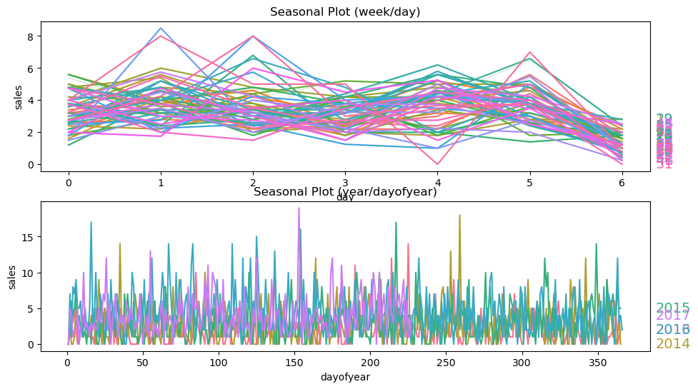
季节规律图

分别按照 weekday 和 year 来绘制季节图。可以看到，在 weekly 上，有比较强的规律性。

X = df_automotive.copy()

# days within a week
X["day"] = X.index.dayofweek  # the x-axis (freq)
X["week"] = X.index.week  # the seasonal period (period)

# days within a year
X["dayofyear"] = X.index.dayofyear
X["year"] = X.index.year
fig, (ax0, ax1) = plt.subplots(2, 1, figsize=(11, 6))
seasonal_plot(X, y="sales", period="week", freq="day", ax=ax0)
seasonal_plot(X, y="sales", period="year", freq="dayofyear", ax=ax1);

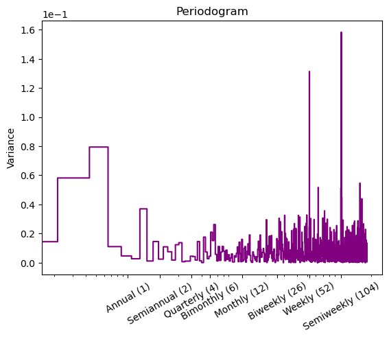
周期图

从周期图里面也可以看到，在 weekly 上有很强的周期性。

plot_periodogram(df_automotive.sales);

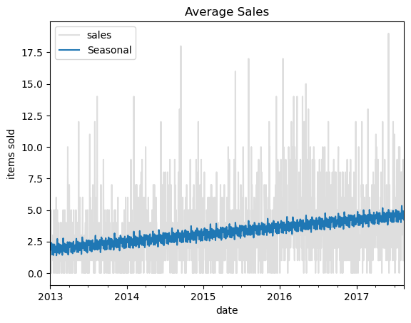
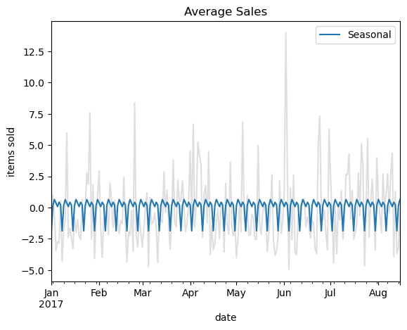
结合大趋势

我们可以结合季节性和趋势，再来预测一次。

from statsmodels.tsa.deterministic import CalendarFourier, DeterministicProcess

fourier = CalendarFourier(freq='M', order=4)
dp = DeterministicProcess(
    index=y.index,
    constant=True,
    order=1,
    seasonal=True,
    additional_terms=[fourier],
    drop=True,
)

X = dp.in_sample()
y = df_automotive["sales"]

model = LinearRegression().fit(X, y)
y_pred = pd.Series(
    model.predict(X),
    index=X.index,
    name='Fitted',
)

y_pred = pd.Series(model.predict(X), index=X.index)
ax = y.plot(**plot_params, alpha=0.5, title="Average Sales", ylabel="items sold")
ax = y_pred.plot(ax=ax, label="Seasonal")
ax.legend();

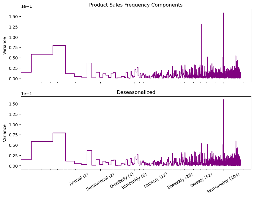
再次查看剩下数据的季节性，可以看到，weekly 上的周期性已经降低了。

y_deseason = y - y_pred

fig, (ax1, ax2) = plt.subplots(2, 1, sharex=True, sharey=True, figsize=(10, 7))
ax1 = plot_periodogram(y, ax=ax1)
ax1.set_title("Product Sales Frequency Components")
ax2 = plot_periodogram(y_deseason, ax=ax2);
ax2.set_title("Deseasonalized");

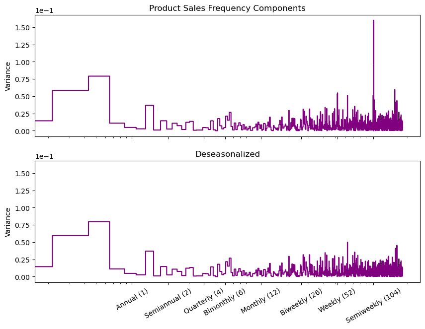
但 Semiweekly 的周期性还保留着，我们可以考虑将其中的傅里叶变换改为是 Weekly，再次学到剩下的季节性。

from statsmodels.tsa.deterministic import CalendarFourier, DeterministicProcess

fourier = CalendarFourier(freq='W', order=7)
dp = DeterministicProcess(
    index=y.index,
    constant=True,
    order=1,
    seasonal=True,
    additional_terms=[fourier],
    drop=True,
)

X = dp.in_sample()

model = LinearRegression().fit(X, y_deseason)
y_pred_1 = pd.Series(
    model.predict(X),
    index=X.index,
    name='Fitted',
)

y_pred_1 = pd.Series(model.predict(X), index=X.index)
ax = y_deseason['2017-01-01':].plot(**plot_params, alpha=0.5, title="Average Sales", ylabel="items sold")
ax = y_pred_1['2017-01-01':].plot(ax=ax, label="Seasonal")
ax.legend();

y_deseason_1 = y_deseason - y_pred_1

fig, (ax1, ax2) = plt.subplots(2, 1, sharex=True, sharey=True, figsize=(10, 7))
ax1 = plot_periodogram(y_deseason, ax=ax1)
ax1.set_title("Product Sales Frequency Components")
ax2 = plot_periodogram(y_deseason_1, ax=ax2);
ax2.set_title("Deseasonalized");

至此，我们已经将季节性学习完毕。

依赖过去的特征

有些模型和过去的目标值有关，我们可以将过去的 target 作为特征，放入模型。

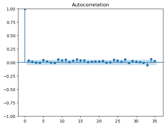
自相关函数 ACF

当前值与滞后值之间的相关程度，包括两个值中间所有项的直接和间接相关信息。

部分相关性函数 PACF

当前值和过去某个滞后之间的相关程度，排除了其他滞后项的影响。

截尾和拖尾

截尾是指大于 k 之后快速趋于 0，拖尾是逐渐下降，最终降到置信区间内。

尝试绘制 ACF 和 PACF 图，发现这两个图都是截尾，即自身的滞后值没有很强的自相关系数。

acf_plot = plot_acf(y_deseason_1, lags=35)
pacf_plot = plot_pacf(y_deseason_1)

残差

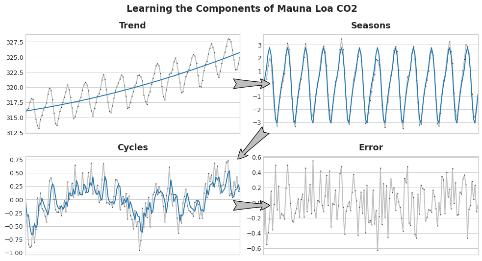
在进行完上面的操作之后，关键的点来了。我们分析了趋势、季节性和周期之后，我们留下一部分残差。

对于残差，一般是用回归模型去预测未来的多个点，比如说，把 y 取后面一天的值，然后进行模型训练。

剩下的工作，基本就是常规的特征工程了。

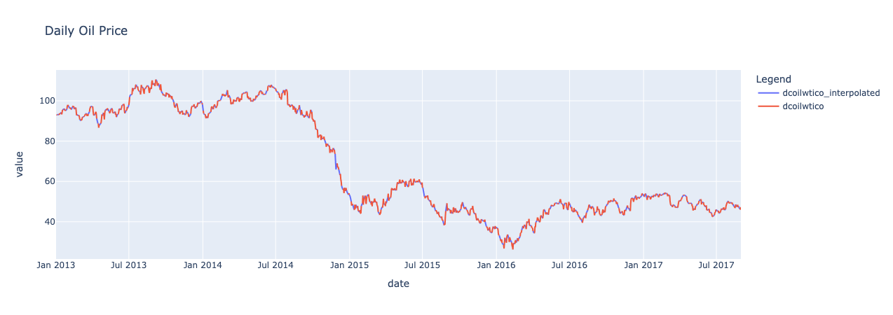
处理油价

油价在周末和放假可能会没有值，需要做一些处理来填补空缺。

# Import
oil = pd.read_csv("oil.csv")
oil["date"] = pd.to_datetime(oil.date)

# 重新采样
oil = oil.set_index("date").dcoilwtico.resample("D").sum().reset_index()

# 填充缺失值

# Interpolate
oil["dcoilwtico"] = np.where(oil["dcoilwtico"] == 0, np.nan, oil["dcoilwtico"])
oil["dcoilwtico_interpolated"] =oil.dcoilwtico.interpolate()

# 进行融合操作并绘制油价图
p = oil.melt(id_vars=['date']), var_name='Legend')
px.line(p.sort_values(["Legend", "date"], ascending = [False, True]), x='date', y='value', color='Legend',title = "Daily Oil Price" )

# 也可以直接从oil绘制油价
oil[['date', 'dcoilwtico_interpolated']].set_index('date').plot(**plot_params)

将油价和数据集关联起来。

df_automotive_sales_ = df_automotive.reset_index().drop(['id', 'store_nbr', 'family', 'time_step', 'lag_1'], axis=1)
df_automotive_sales_['date'] = pd.to_datetime(oil.date)
df_automotive_sales = pd.merge(df_automotive_sales_, oil, how='left')
df_automotive_sales.drop(['dcoilwtico'], axis=1, inplace=True)

处理假日

处理假日有很多需要注意的，比如国外有桥假的概念，即周四放假的话，会额外多放一天周五（桥假），连上周末一起放。还有调假，国家/州/城市假。

holidays = pd.read_csv("holidays_events.csv")
holidays["date"] = pd.to_datetime(holidays.date)

# holidays[holidays.type == "Holiday"]
# holidays[(holidays.type == "Holiday") & (holidays.transferred == True)]

# Transferred Holidays
tr1 = holidays[(holidays.type == "Holiday") & (holidays.transferred == True)].drop("transferred", axis = 1).reset_index(drop = True)
tr2 = holidays[(holidays.type == "Transfer")].drop("transferred", axis = 1).reset_index(drop = True)
tr = pd.concat([tr1,tr2], axis = 1)

tr = tr.iloc[:, [5,1,2,3,4]]
holidays = holidays[(holidays.transferred == False) & (holidays.type != "Transfer")].drop("transferred", axis = 1)
holidays = pd.concat([holidays,tr]).reset_index(drop = True)

# Additional Holidays
holidays["description"] = holidays["description"].str.replace("-", "").str.replace("+", "").str.replace('\d+', '')
holidays["type"] = np.where(holidays["type"] == "Additional", "Holiday", holidays["type"])

# Bridge Holidays
holidays["description"] = holidays["description"].str.replace("Puente ", "")
holidays["type"] = np.where(holidays["type"] == "Bridge", "Holiday", holidays["type"])


# Work Day Holidays, that is meant to payback the Bridge.
work_day = holidays[holidays.type == "Work Day"]
holidays = holidays[holidays.type != "Work Day"]

此外还是各种事件，比如火山爆发，地震，大型庆祝活动。

events = holidays[holidays.type == "Event"].drop(["type", "locale", "locale_name"], axis = 1).rename({"description":"events"}, axis = 1)
events
holidays = holidays[holidays.type != "Event"].drop("type", axis = 1)

继续拆分各个州的假期，城市的假期，后面会根据超市所在的地区做关联

regional = holidays[holidays.locale == "Regional"].rename({"locale_name":"state", "description":"holiday_regional"}, axis = 1).drop("locale", axis = 1).drop_duplicates()
national = holidays[holidays.locale == "National"].rename({"description":"holiday_national"}, axis = 1).drop(["locale", "locale_name"], axis = 1).drop_duplicates()
local = holidays[holidays.locale == "Local"].rename({"description":"holiday_local", "locale_name":"city"}, axis = 1).drop("locale", axis = 1).drop_duplicates()

关联 store 所在地区

stores = pd.read_csv('stores.csv')
df_automotive_sales_stores = pd.merge(df_automotive_sales, stores[stores['store_nbr'] == 1])
df_automotive_sales_stores = pd.merge(df_automotive_sales_stores, national, how = "left")
# Regional
df_automotive_sales_stores = pd.merge(df_automotive_sales_stores, regional, how = "left", on = ["date", "state"])
# Local
df_automotive_sales_stores = pd.merge(df_automotive_sales_stores, local, how = "left", on = ["date", "city"])

处理工作日

df_automotive_sales_stores = pd.merge(df_automotive_sales_stores,  work_day[["date", "type"]].rename({"type":"IsWorkDay"}, axis = 1),how = "left")

处理巴西世界杯

events["events"] =np.where(events.events.str.contains("futbol"), "Futbol", events.events)

对 events 进行独热编码

def one_hot_encoder(df, nan_as_category=True):
    original_columns = list(df.columns)
    categorical_columns = df.select_dtypes(["category", "object"]).columns.tolist()
    # categorical_columns = [col for col in df.columns if df[col].dtype == 'object']
    df = pd.get_dummies(df, columns=categorical_columns, dummy_na=nan_as_category)
    new_columns = [c for c in df.columns if c not in original_columns]
    df.columns = df.columns.str.replace(" ", "_")
    return df, df.columns.tolist()

events, events_cat = one_hot_encoder(events, nan_as_category=False)
events["events_Dia_de_la_Madre"] = np.where(events.date == "2016-05-08", 1,events["events_Dia_de_la_Madre"])
events = events.drop(239)

df_automotive_sales_stores = pd.merge(df_automotive_sales_stores, events, how = "left")
df_automotive_sales_stores[events_cat] = df_automotive_sales_stores[events_cat].fillna(0)

df_automotive_sales_stores.head()

对假日进行独热编码

d = df_automotive_sales_stores

d["holiday_national_binary"] = np.where(d.holiday_national.notnull(), 1, 0)
d["holiday_local_binary"] = np.where(d.holiday_local.notnull(), 1, 0)
d["holiday_regional_binary"] = np.where(d.holiday_regional.notnull(), 1, 0)

#
d["national_independence"] = np.where(d.holiday_national.isin(['Batalla de Pichincha',  'Independencia de Cuenca', 'Independencia de Guayaquil', 'Independencia de Guayaquil', 'Primer Grito de Independencia']), 1, 0)
d["local_cantonizacio"] = np.where(d.holiday_local.str.contains("Cantonizacio"), 1, 0)
d["local_fundacion"] = np.where(d.holiday_local.str.contains("Fundacion"), 1, 0)
d["local_independencia"] = np.where(d.holiday_local.str.contains("Independencia"), 1, 0)


holidays, holidays_cat = one_hot_encoder(d[["holiday_national","holiday_regional","holiday_local"]], nan_as_category=False)
d = pd.concat([d.drop(["holiday_national","holiday_regional","holiday_local"], axis = 1),holidays], axis = 1)

he_cols = d.columns[d.columns.str.startswith("events")].tolist() + d.columns[d.columns.str.startswith("holiday")].tolist() + d.columns[d.columns.str.startswith("national")].tolist()+ d.columns[d.columns.str.startswith("local")].tolist()
d[he_cols] = d[he_cols].astype("int8")

d.head()

创建真正的 workday

# Time Related Features
def create_date_features(df):
    df['month'] = df.date.dt.month.astype("int8")
    df['day_of_month'] = df.date.dt.day.astype("int8")
    df['day_of_year'] = df.date.dt.dayofyear.astype("int16")
    df['week_of_month'] = (df.date.apply(lambda d: (d.day-1) // 7 + 1)).astype("int8")
    df['week_of_year'] = (df.date.dt.isocalendar().week).astype("int8")
    df['day_of_week'] = (df.date.dt.dayofweek + 1).astype("int8")
    df['year'] = df.date.dt.year.astype("int32")
    df["is_wknd"] = (df.date.dt.weekday // 4).astype("int8")
    df["quarter"] = df.date.dt.quarter.astype("int8")
    df['is_month_start'] = df.date.dt.is_month_start.astype("int8")
    df['is_month_end'] = df.date.dt.is_month_end.astype("int8")
    df['is_quarter_start'] = df.date.dt.is_quarter_start.astype("int8")
    df['is_quarter_end'] = df.date.dt.is_quarter_end.astype("int8")
    df['is_year_start'] = df.date.dt.is_year_start.astype("int8")
    df['is_year_end'] = df.date.dt.is_year_end.astype("int8")
    # 0: Winter - 1: Spring - 2: Summer - 3: Fall
    df["season"] = np.where(df.month.isin([12,1,2]), 0, 1)
    df["season"] = np.where(df.month.isin([6,7,8]), 2, df["season"])
    df["season"] = pd.Series(np.where(df.month.isin([9, 10, 11]), 3, df["season"])).astype("int8")
    return df
d = create_date_features(d)




# Workday column
d["workday"] = np.where((d.holiday_national_binary == 1) | (d.holiday_local_binary==1) | (d.holiday_regional_binary==1) | (d['day_of_week'].isin([6,7])), 0, 1)
d["workday"] = pd.Series(np.where(d.IsWorkDay.notnull(), 1, d["workday"])).astype("int8")
d.drop("IsWorkDay", axis = 1, inplace = True)

# Wages in the public sector are paid every two weeks on the 15 th and on the last day of the month.
# Supermarket sales could be affected by this.
d["wageday"] = pd.Series(np.where((d['is_month_end'] == 1) | (d["day_of_month"] == 15), 1, 0)).astype("int8")

d.head(15)

接下来就是拆分数据集，做回归预测并看 RMSE，这里就不写了。

个人想法

前前后后，断断续续地一个月总算把这块看完了，但其实还是很片面，很多时间花在特征工程上去了。关于时间序列还有其他的模型可以用，尝试使用几个常见的模型。但是，就学习时间序列预测来说，这道题实在不太适合，太多的特征工程了。